
RAG Architect’s Handbook
A Deep Dive into Next-Gen RAG Patterns


If you have been building with Large Language Models over the last two years, you have likely walked the same path as the rest of us. You started with a simple API call to GPT-5 or similar. Then, you realized the model didn’t know about your company’s private data or the events of last week. So, you built a simple Retrieval-Augmented Generation (RAG) pipeline: chunk a PDF, throw it into a vector database, look up the top-3 similar chunks, and feed them to the LLM. It felt like magic until you put it into production.
Suddenly, the cracks appeared. Users asked vague questions, and the vector search returned noise. They asked complex comparison questions, and the system failed because the answer wasn’t in a single chunk. Or worse, the model confidently hallucinated an answer based on irrelevant retrieval results.
We are now in the Post-Naive RAG era. The industry has moved beyond simple semantic search into complex, architectural patterns designed to handle ambiguity, reason over data, and self-correct. We aren’t just building pipelines anymore; we are building cognitive architectures.
This post is a deep technical dive into these emerging architectures. We will look at GraphRAG, which structures data for global reasoning; Speculative RAG, which trades compute for speed and accuracy; Agentic RAG, which gives the model autonomy; and Adaptive RAG, which routes traffic like a smart load balancer. We will explore the why and how of each pattern, looking at the algorithms, the implementation strategies, and the hard trade-offs you will face as a developer.
Naive RAG and the Bag of Chunks Problem
Before we appreciate the complex architectures, we need to understand exactly why the baseline fails. Naive RAG is the standard Retrieve-then-Generate workflow.
The Architecture
The workflow is linear and rigid
Indexing: You take your documents, split them into fixed-size chunks (e.g., 512 tokens), and embed them using a model like OpenAI’s text-embedding-3-small or similar
Retrieval: The user’s query is embedded. You perform a k-Nearest Neighbors search in the vector space using Cosine Similarity.
Generation: You take the top k chunks (usually 3 to 5), paste them into a prompt template and hit the LLM generation endpoint.
While this works for simple lookup tasks, it treats knowledge as a bag of chunks and can lead to a couple of problems
Semantic Mismatch: A user might ask, “What goes wrong when the engine overheats?” The document might say, “Thermal throttling induces system shutdown.” A naive vector search might miss this connection if the embedding model hasn’t seen that specific terminology linkage.
The Lost in the Middle Phenomenon: LLMs are not perfect readers. Research shows that models tend to focus on the beginning and end of their context window. If the crucial answer is buried in the middle of retrieved chunk #3 out of 5, the model might ignore it.
Lack of Global Context: If you ask, “What are the main themes in this 100-page report?”, Naive RAG fails. It will retrieve 5 random chunks mentioning “themes” or specific details, but it cannot “read” the whole document to synthesize a summary. It suffers from a narrow field of view.
These limitations have driven the research community to develop the Advanced and Modular patterns we will discuss next.
Pre-Retrieval Optimization
The first line of defense against bad RAG performance is better inputs. If the user asks a bad question, a vector database will give you bad answers. Pre-retrieval strategies focus on Query Transformation - rewriting the user’s intent into a format the machine understands better.
RAG-Fusion: Multi-Query Triangulation
One of the most robust patterns to emerge is RAG-Fusion. It addresses the problem of user queries being too specific, too vague, or just poorly phrased.
The Developer’s Perspective: Imagine a user asks, “Why is the system slow?” In your vector DB, the relevant docs might be about “latency,” “throughput bottlenecks,” or “database locking.” A single query for “slow” might miss the “locking” document entirely.
How RAG-Fusion Works
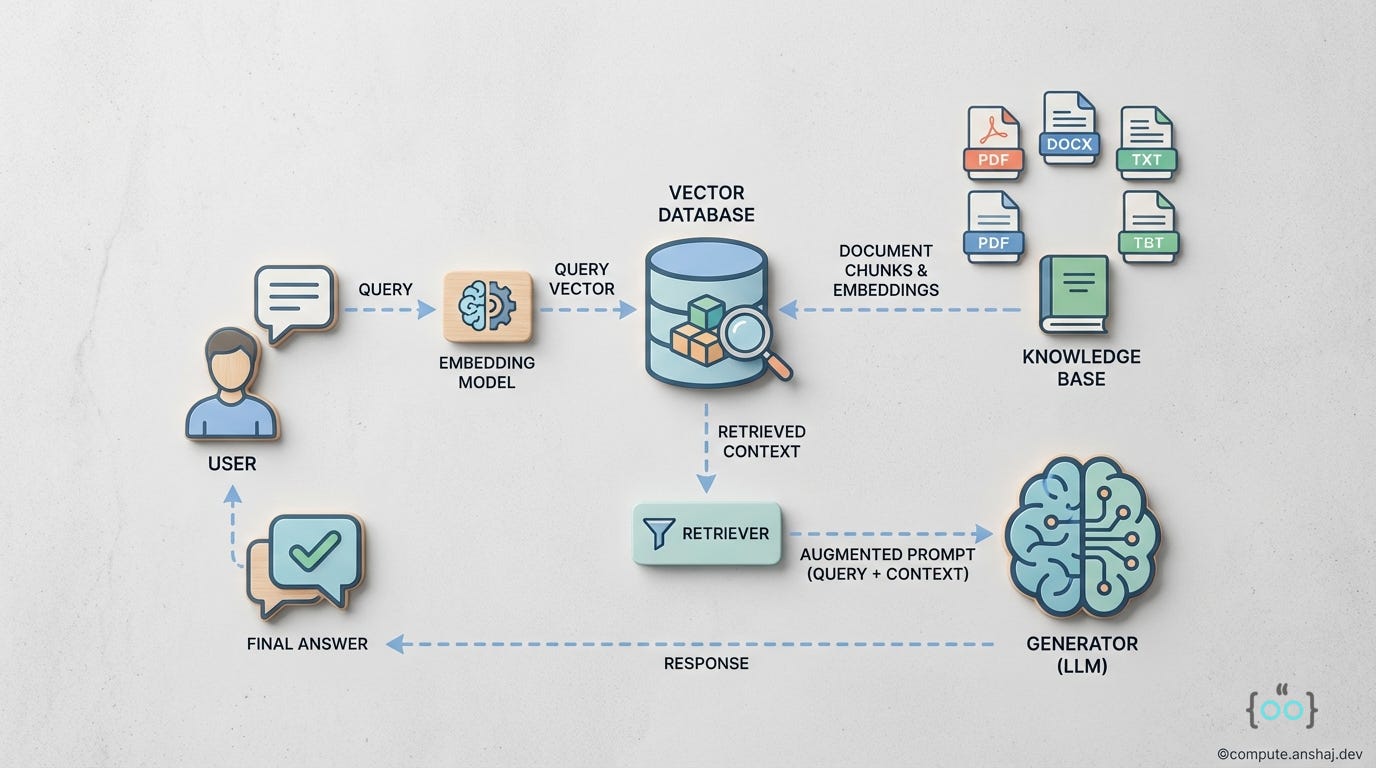
Query Generation: Instead of searching for the user’s raw query, we use an LLM to generate N (usually 3-5) variations of that query from different perspectives.
User Query: “Why is the system slow?”
Generated Q1: “Common causes of latency in the application.”
Generated Q2: “Database locking and performance bottlenecks.”
Generated Q3: “Network throughput issues in the infrastructure.”
Parallel Vector Search: We run all these queries against the vector database. This casts a wider net, retrieving a diverse set of documents that might not overlap.
Reciprocal Rank Fusion (RRF): Now we have 5 lists of documents. We don’t just append them; we fuse them. RRF is a standard algorithm from information retrieval that ranks documents based on their position in multiple lists. If “Doc A” appears in the top 3 for all generated queries, it’s highly likely to be relevant.
The score for a document d is calculated as:
where k is a smoothing constant (often 60) and rq(d) is the rank of the document in query q’s list.
✨ Implementation Note ✨
This increases your retrieval latency because you are making N vector DB calls (though you can do them in parallel). However, the increase in recall (finding the right document) is often worth the extra milliseconds.
HyDE: Hypothetical Document Embeddings
HyDE takes a fascinating approach: “Fake it till you make it.”
The Problem: Vector search works best when the query and the document look similar. But a question (”How do I reset my password?”) looks very different from a procedural document (”To initiate a credential reset, navigate to settings...”). They have different lengths, structures, and vocabularies. This is the semantic gap.
The HyDE Solution
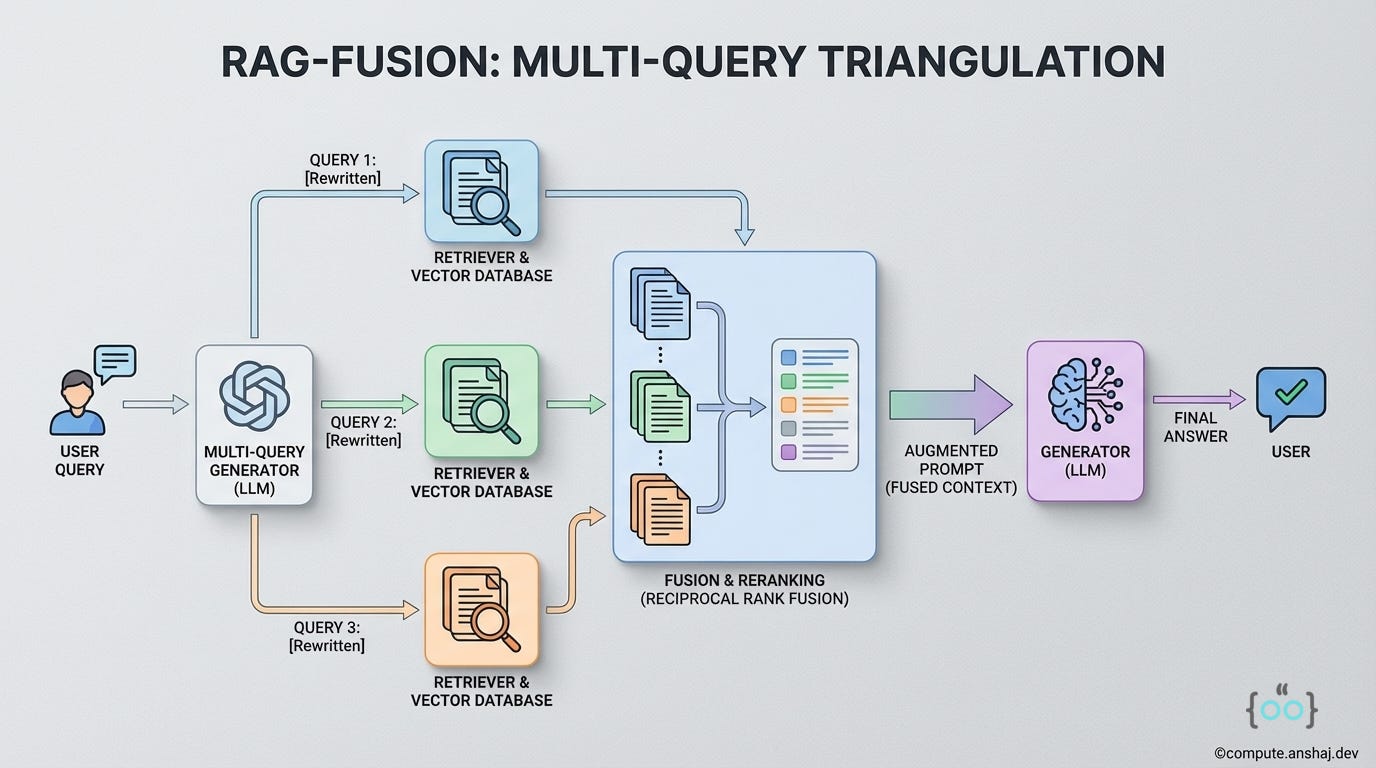
Hallucinate an Answer: We ask an LLM to write a hypothetical answer to the user’s question. We don’t care if the facts are wrong; we care about the patterns.
Prompt: “Write a short passage explaining how to reset a password in this system.”
Hypothetical Doc: “To reset your password, go to the user profile tab, click on security settings, and select the ‘Forgot Password’ link. You will receive an email...”
Embed the Hallucination: We encode this hypothetical document into a vector.
Retrieve Real Documents: We search the vector DB using this vector.
The hypothetical document is semantically much closer to the real manual than the user’s short question was. It acts as a bridge. HyDE aligns the retrieval task to be Answer-to-Answer rather than Question-to-Answer.
✨ Implementation Note ✨
If the LLM hallucinates something completely off-base (e.g., it invents a feature that doesn’t exist), the vector search will look for documents about that non-existent feature, leading to a total retrieval failure.7 HyDE is powerful but risky for domain-specific queries where the LLM has no prior training (e.g., proprietary internal APIs).
Semantic Routing
Sometimes, you don’t need RAG at all. If a user says “Hi”, retrieving documents is a waste of money. Semantic Routing acts as a traffic controller.
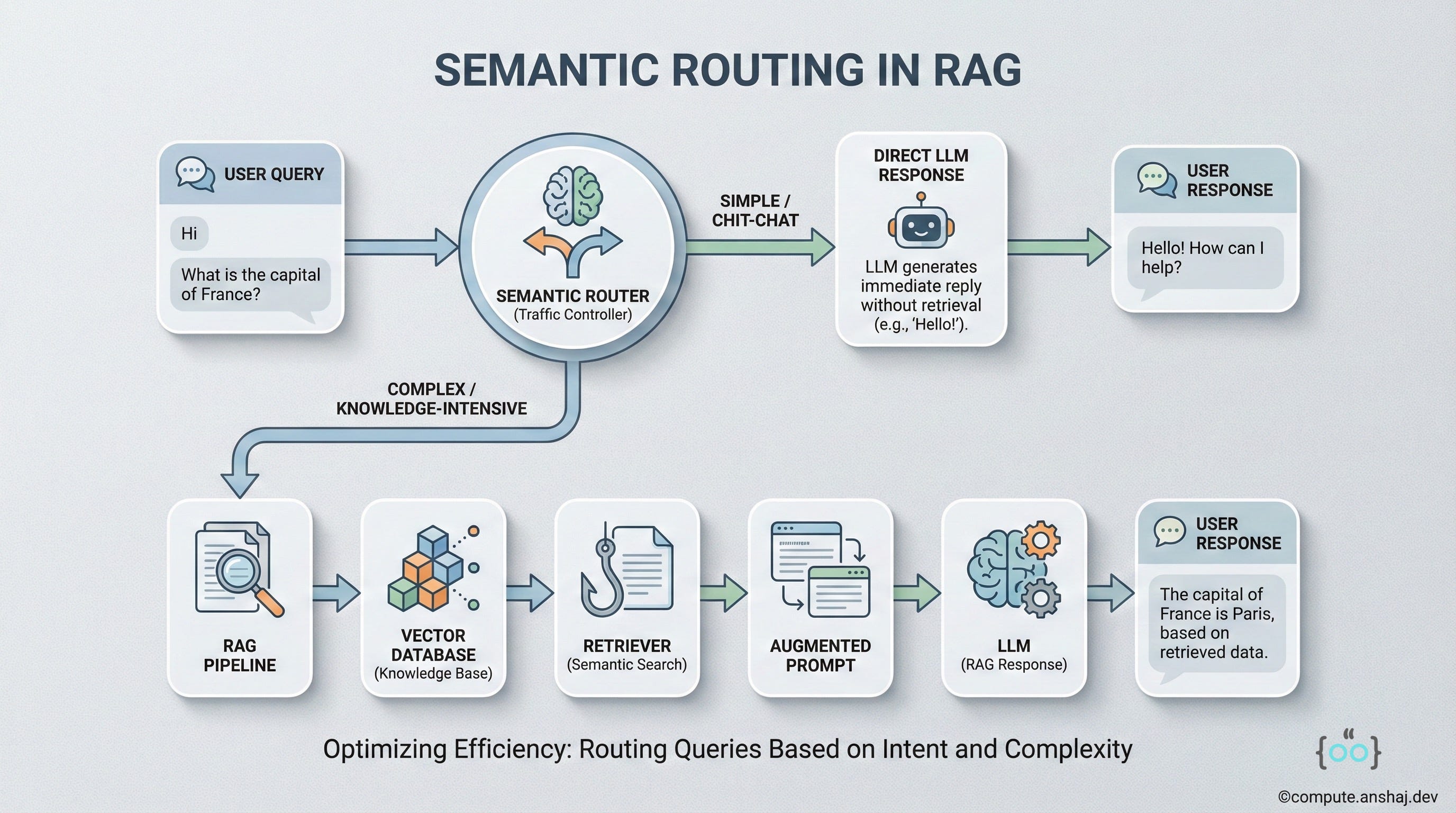
The mechanism works as such. You train a classifier (or use a zero-shot LLM call) to categorize the incoming query into buckets:
Chit-chat: Route to a simple LLM (no RAG).
Fact Retrieval: Route to Vector Search.
Summarization: Route to a specialized summarization pipeline.
Coding: Route to a code-specialized model.
This is the first step towards Adaptive RAG, which we will discuss later. It prevents the system from blindly running expensive retrieval pipelines for every input.
Post-Retrieval Optimization
Once you have retrieved a set of documents, your job isn’t done. The raw results from a vector database are often noisy. You might get 20 documents, but only 3 are useful. Post-retrieval steps refine this context.
Reranking: The Quality Filter
This is arguably the highest ROI upgrade you can make to a Naive RAG system.
Regular Vector search is fast but fuzzy. It compresses all meaning into a single vector. A Cross-Encoder is a different type of model (like a BERT classifier) that takes a pair of texts (Query, Document) and outputs a similarity score from 0 to 1.10
The Workflow
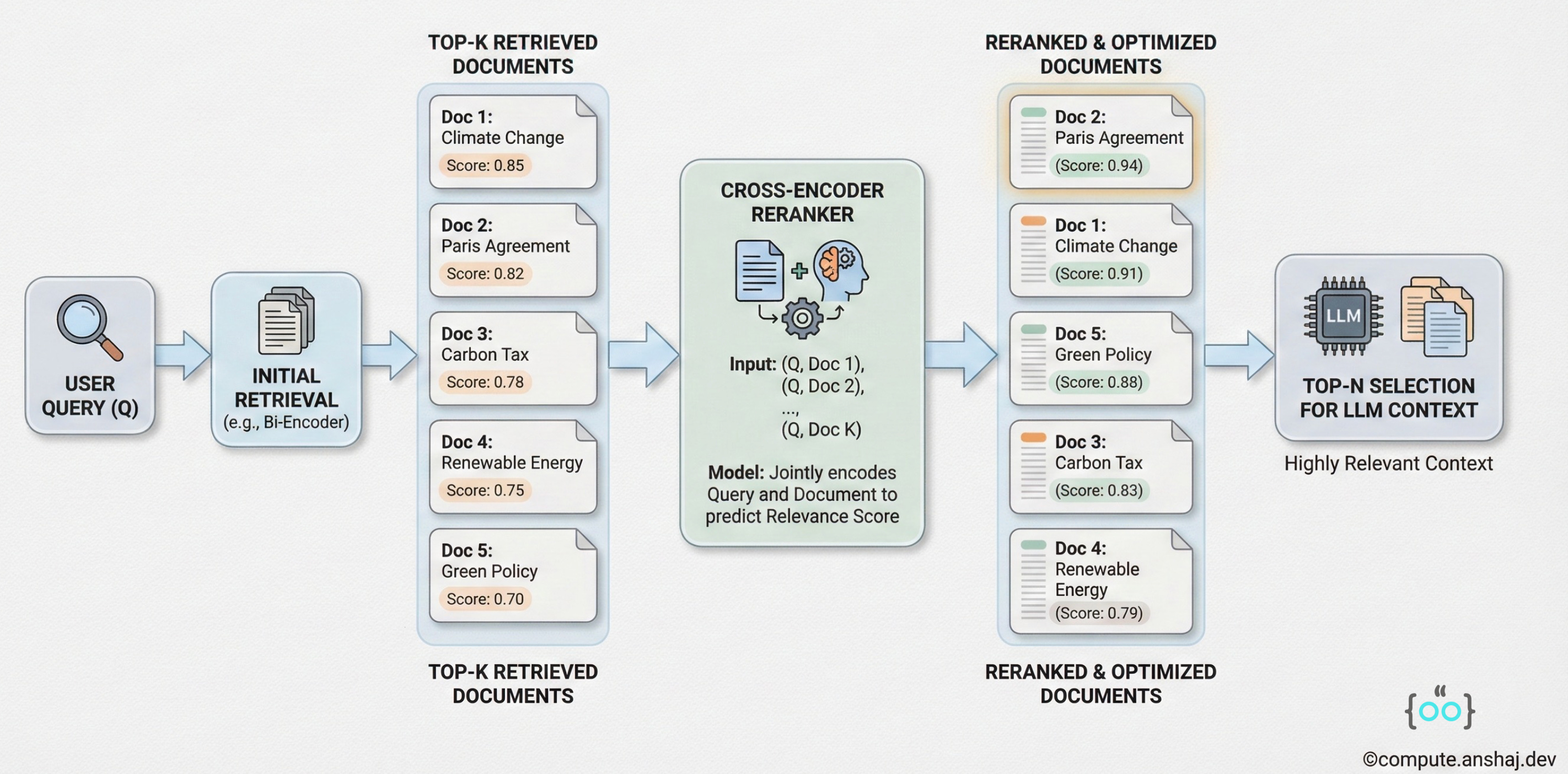
Retrieve Wide: Instead of getting top-5 documents, get top-50 from the vector DB.
Rerank: Pass all 50 pairs (Query + fetched documents) through the Cross-Encoder.
Sort and Slice: Sort by the new score and take the top-5.
Cross-Encoders are much more accurate than vector similarity because they can “pay attention” to the interaction between specific words in the query and the document. The trade-off is latency - running a Cross-Encoder on 50 documents takes significantly longer than a vector lookup. But for precision-critical apps (like legal search), it is non-negotiable.
Context Compression and Selection
Feeding 10,000 tokens of context to the LLMs is expensive and slow. Context Compression helps to reduce this load without losing information.
Couple of techniques that help us do this are:
LLMChainExtractor: Using a smaller LLM to read the retrieved document and extract only the sentences relevant to the query, discarding the rest.
Embeddings-based Filtering: Removing documents that are below a certain similarity threshold (e.g., discarding anything with a cosine similarity < 0.7).
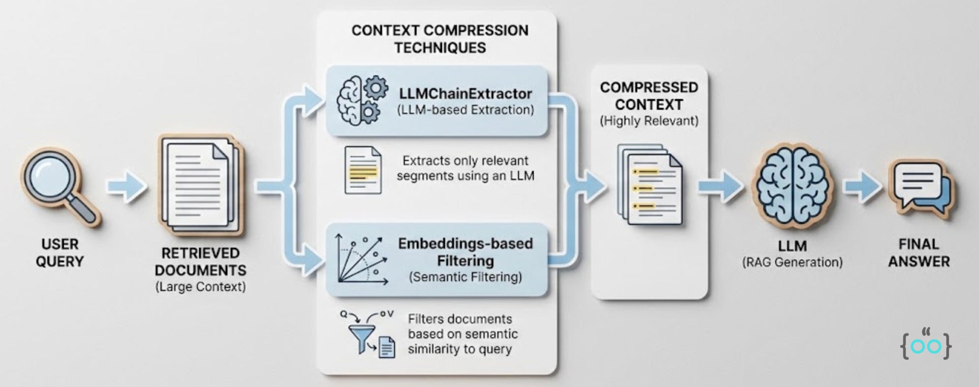
This ensures that the final prompt sent to the generator is dense with signal and low on noise, which reduces hallucination risks.
GraphRAG
GraphRAG fundamentally changes how we index data. It moves away from flat lists of text chunks and towards structured relationships.
Vector RAG is great for “Needle in a Haystack” queries. It is terrible for Global Understanding queries. If you ask, “How do the relationships between the factions in this story evolve?” a vector search will find you snippets where factions are mentioned. It won’t find you the evolution or the structure of the conflict.
Building the Graph
GraphRAG, specifically the approach championed by Microsoft Research, uses an LLM to build a Knowledge Graph (KG) during the indexing phase.
The Pipeline
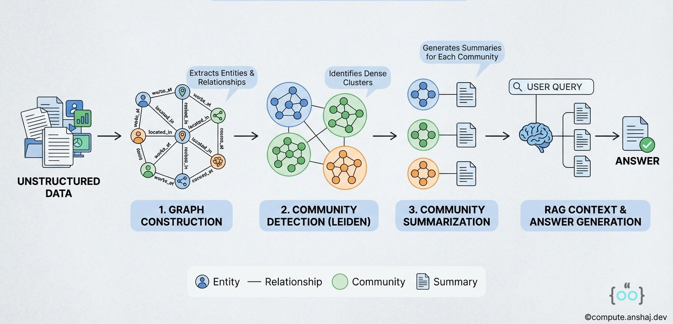
Source Parsing: Documents are split into chunks.
Extraction: An LLM processes each chunk to extract Entities (People, Places, Organizations) and Relationships(e.g., “Person A works for Organization B”).
Graph Construction: These form a graph structure (Nodes and Edges) stored in a graph database like Neo4j.
Community Detection: This is the sauce. The system uses algorithms like Leiden (a hierarchical clustering algorithm) to group nodes into communities.
Level 0: All nodes.
Level 1: Broad clusters (e.g., “Tech Companies,” “Regulatory Bodies”).
Level 2: Tighter clusters (e.g., “AI Startups in SF”).
Community Summarization: The LLM generates a summary for each community.
Global Search Mechanism
When a user asks a high-level question (”What are the major market trends in this dataset?”):
The system does not search the raw text chunks.
It searches the Community Summaries.
Because these summaries are hierarchical, the system can answer at the appropriate level of abstraction.
It synthesizes these summaries into a global answer.
✨ Implementation Note ✨
The Pros of a Graph RAG include unmatched ability to answer thematic, multi-hop, and global questions. It structures unstructured data.
While the cons revolve around Cost and Complexity. Building the graph is expensive (lots of LLM calls). Maintaining it when new documents are added is non-trivial. It adds a heavy preprocessing step before the first query can even be answered.
Speculative RAG: Need for Speed
In production, latency is a killer. Users may dislike waiting 5 seconds for an answer. Speculative RAG is an architectural pattern designed to break the linear dependency of standard RAG to speed things up. It borrows the idea of “Speculative Decoding” from model optimization. The core idea is to separate the drafting of an answer from the verification of it.
The Roles
The Drafter (Specialist): A smaller, faster, perhaps fine-tuned model (e.g., Llama-3-8B).
The Verifier (Generalist): A larger, smarter model (e.g., GPT-5).
The Workflow
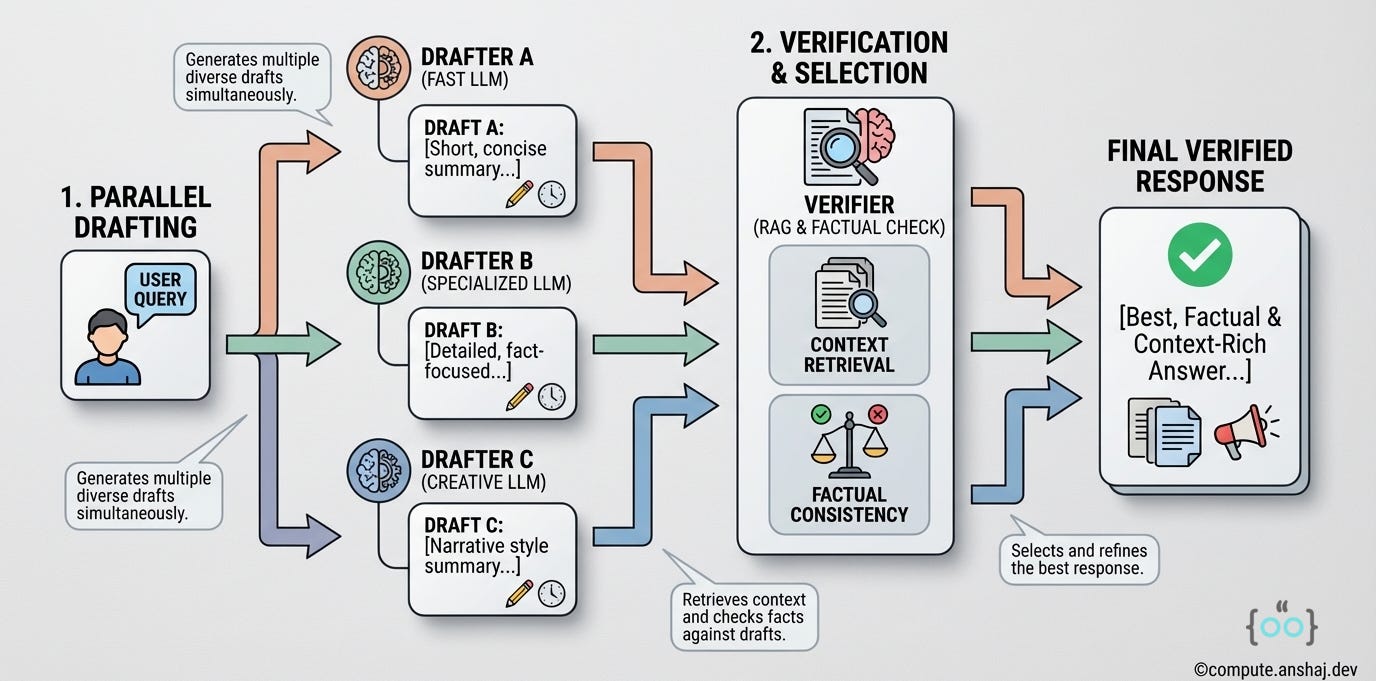
Parallel Drafting: Instead of one large prompt, we split our retrieved documents into subsets (e.g., 4 subsets of 2 docs each). We spawn 4 instances of the Drafter model in parallel. Each Drafter reads its small subset and generates a draft answer.
Verification: The Verifier looks at the question and the 4 draft answers. It doesn’t necessarily need to read all the original documents (saving tokens). It evaluates the drafts for consistency and rationale.
Selection: The Verifier picks the best draft or synthesizes them into a final answer.
You might think running 4 models is slower than 1. But because the Drafters run in parallel and use smaller context windows (fewer tokens), the Time to First Token and overall generation time can be significantly lower.
Research benchmarks on datasets like PubHealth show Speculative RAG can reduce latency by over 50% while actually increasing accuracy (by ~13%). The accuracy gain comes from the ensemble effect (remember Random Forests?) - multiple drafters looking at data from different angles reduce the chance of the model fixating on a single wrong detail.
The Critic: Self-Correcting Architectures
One of the biggest fears in RAG deployment is of Silent Failure. The system retrieves garbage, the LLM hallucinates an answer based on that garbage, and the user believes it. Self-Correcting RAG adds a feedback loop to catch these errors.
Corrective RAG (CRAG)
CRAG adds a lightweight Retrieval Evaluator (Relevance Checker) into the pipeline.
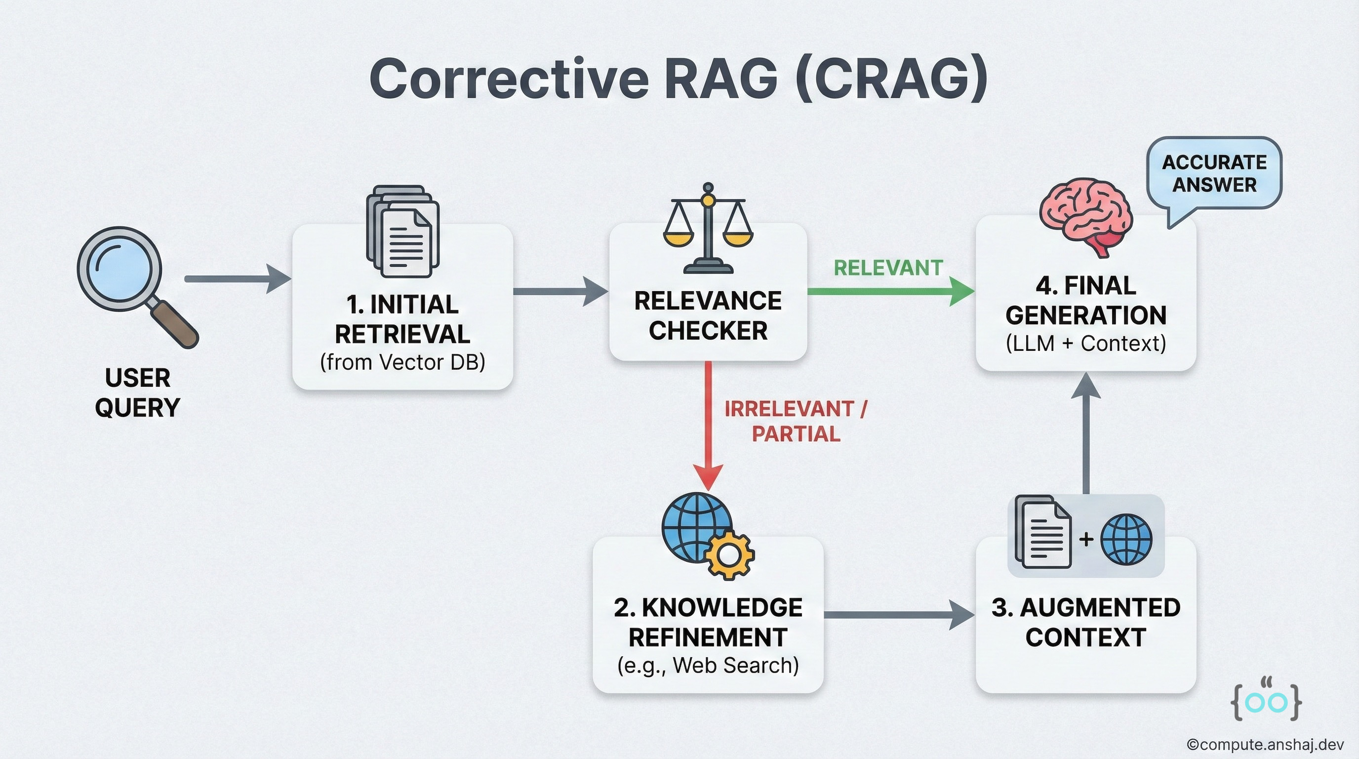
The Logic
Retrieve: Get documents.
Evaluate: A specialized model (often a T5 or small BERT-sized model) scores the relevance of the documents to the query.
Branching Decision:
Correct (High Confidence): Proceed to generation. Strip out irrelevant snippets.
Incorrect (Low Confidence): The retrieved docs are trash. Fallback: Trigger a web search or check a backup knowledge base. Do not use the bad docs.
Ambiguous: Combine the retrieved docs with a web search to fill in the gaps.
This simple Traffic Light - like system prevents the generator from ever seeing purely irrelevant context, which is the primary cause of hallucinations.
Self-RAG: Reflection Tokens
Self-RAG takes a different approach. Instead of an external evaluator, it trains the Generator LLM to critique itself.
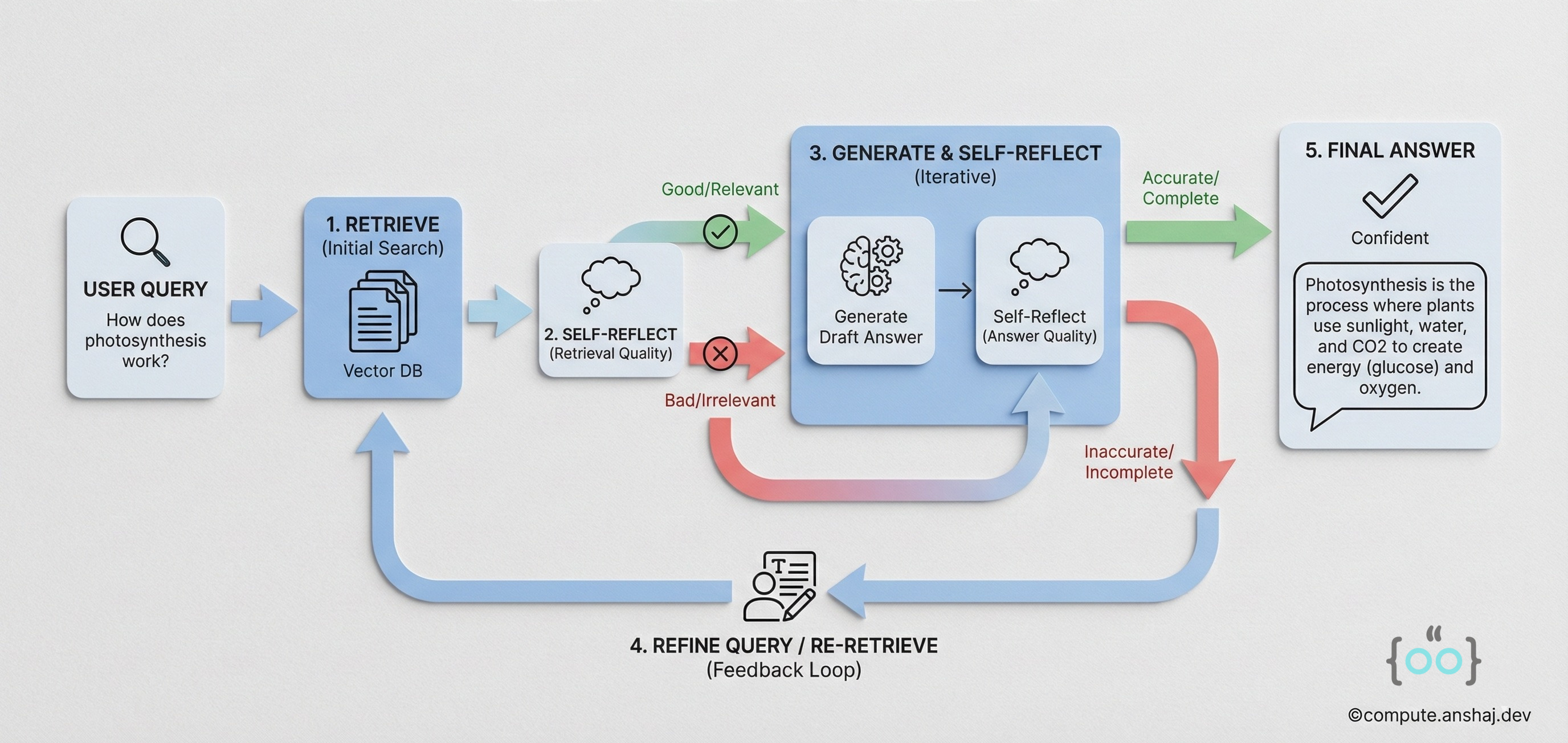
Reflection Tokens: The model is fine-tuned to emit special tokens inside its generation stream:
“I need more data for this next sentence.”
“The document I just read is irrelevant.”
“The sentence I just wrote is not supported by the evidence.”
“This answer is useful for the user.”.
During inference, the model generates a thought, critiques it with a token, and if the token is negative (e.g., = False), it backtracks and regenerates. This happens at the token/sentence level, offering much finer-grained control than CRAG’s document-level filtering.
However, implementation is harder: you typically need to fine-tune your own model or use a specifically trained Self-RAG checkpoint
Adaptive RAG: The Manager
Adaptive RAG is about efficiency. Not every query needs a $0.05 web search and a complex graph traversal. Some queries just need a quick lookup. Adaptive RAG uses a Classifier to route queries to the cheapest effective pipeline.
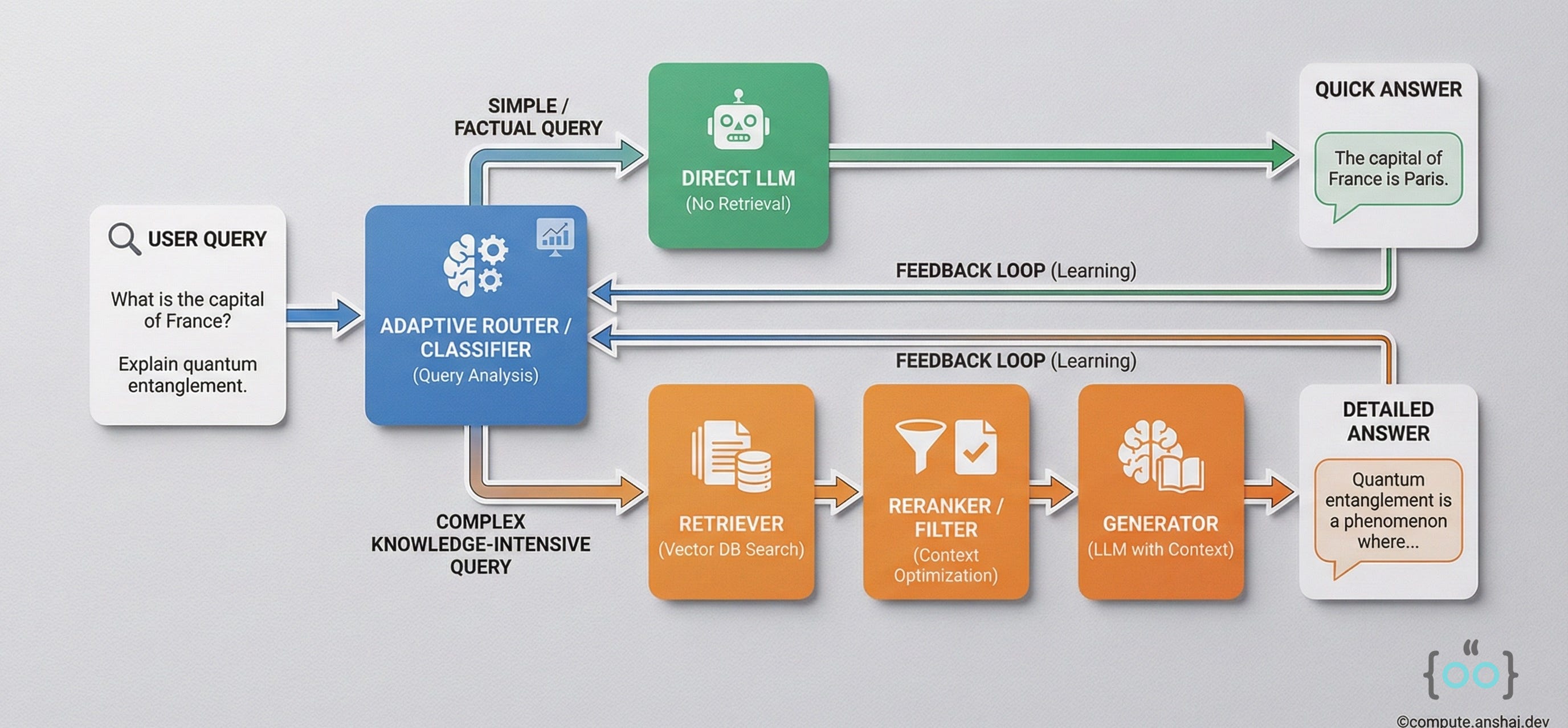
Complexity Classification
The router analyzes the query and assigns a complexity level:
Simple (No Retrieval): “What is the capital of France?” -> Let the LLM answer from memory. Fast, free.
Moderate (Single-Step): “Who is the CEO of LangChain?” -> Vector Search -> Generate.
Complex (Multi-Step): “Compare the battery life of the iPhone 17 vs. Pixel 10 based on recent reviews.” -> This requires retrieving reviews for both, normalizing the data, and synthesizing.
Dynamic Routing Logic
In a framework like LangChain or LangGraph, you implement this as a conditional chain.
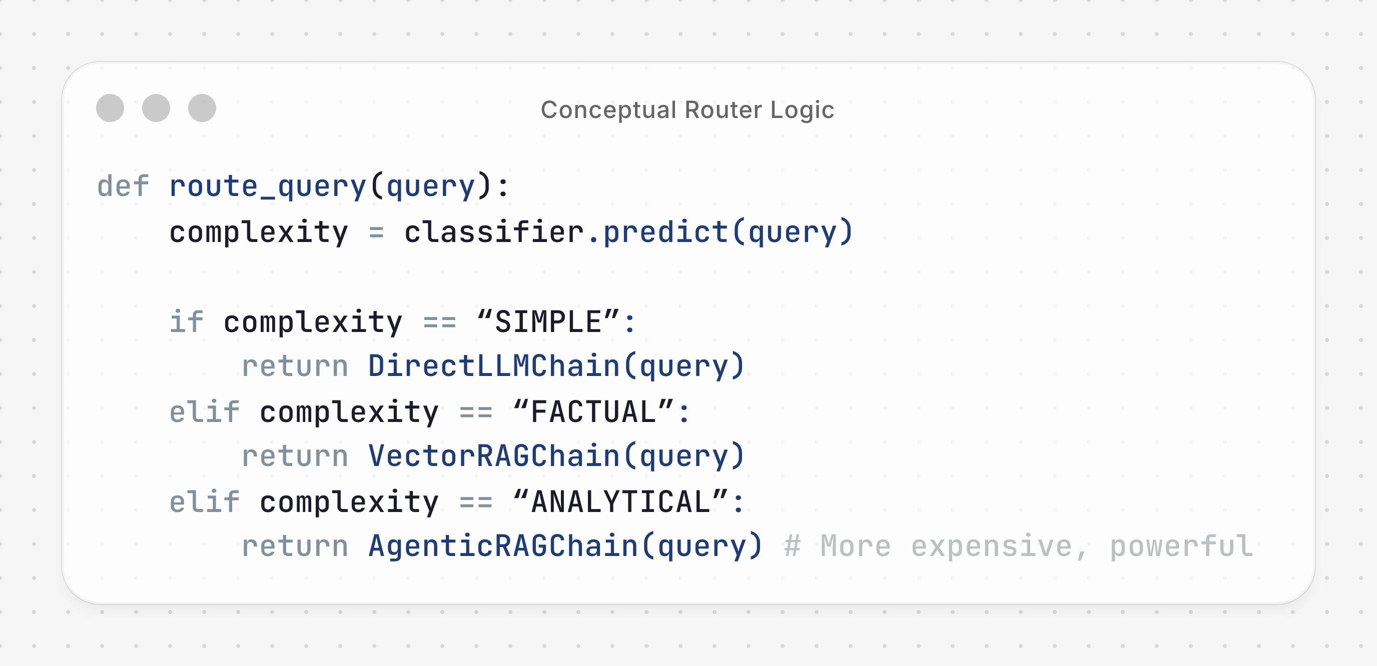
This architecture is critical for scaling. It optimizes your “Token Budget.” You spend your expensive compute only on the hard problems.
Tree of Clarifications
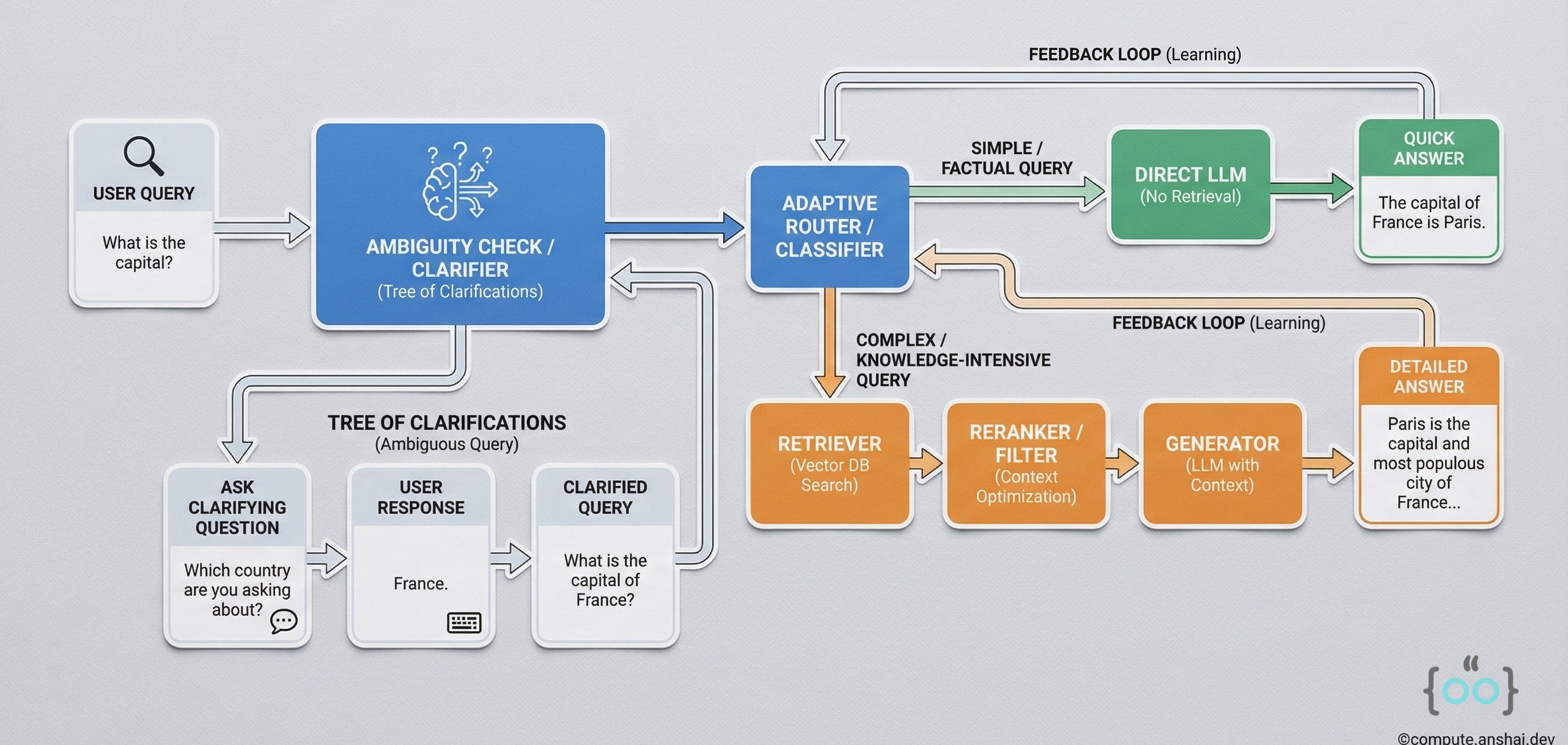
A sub-pattern of adaptive RAG handles Ambiguity. If a user asks “Who won the game?”, Adaptive RAG shouldn’t guess. The Tree of Clarifications architecture generates disambiguating questions (”Did you mean the NBA game last night or the World Cup final?”), constructs a tree of possible paths, retrieves info for each, and prunes the dead ends.
The Autonomous: Agentic RAG
If Adaptive RAG is a manager, Agentic RAG is an autonomous worker. It moves beyond pipelines (DAGs) to loops (Cyclic Graphs). This is the current frontier of RAG development.
The ReAct Loop
The core of Agentic RAG is the ReAct (Reason + Act) pattern.
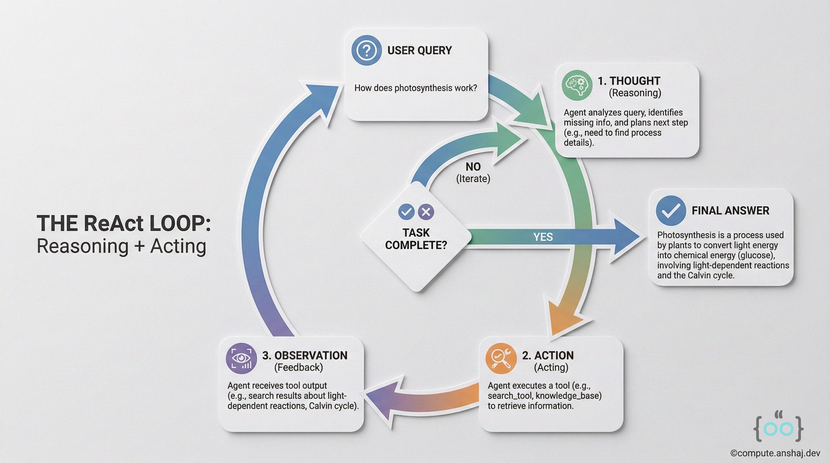
The agent doesn’t just retrieve; it thinks.
Thought: The user wants to compare two stocks. I need the price of AAPL first.
Action: Call Tool get_stock_price(”AAPL”).
Observation: AAPL is $150.
Thought: Now I need the price of MSFT.
Action: Call Tool get_stock_price(”MSFT”).
Observation: MSFT is $300.
Thought: I have both. Now I will compare.
Final Answer: MSFT is double the price of AAPL.
Tool Use and Autonomy
In Agentic RAG, the “Retriever” is just one tool in a toolkit that might also include:
Web Search (for real-time data).
Calculator (for math, where LLMs fail).
SQL Connector (for structured DBs).
The agent decides when to use the retriever. If the first retrieval is bad, the agent can observe that (”I didn’t find the answer”) and decide to rewrite the query and try again. This Retry Loop is what makes Agentic RAG so powerful—and so dangerous (infinite loops are possible!). For more on this, you can read my article below on AI agent tooling.

Chain-of-Note: Noise control
We talked about noise earlier, but Chain-of-Note (CoN) deserves its own section as a specific architectural remedy for the “Unknown” problem.
The Problem: Standard RAG is terrified of saying “I don’t know.” If you ask “Who is the King of Mars?” and the retriever brings back a document about the “King of Burgers,” a standard RAG model might hallucinate “The King of Mars is the King of Burgers.”
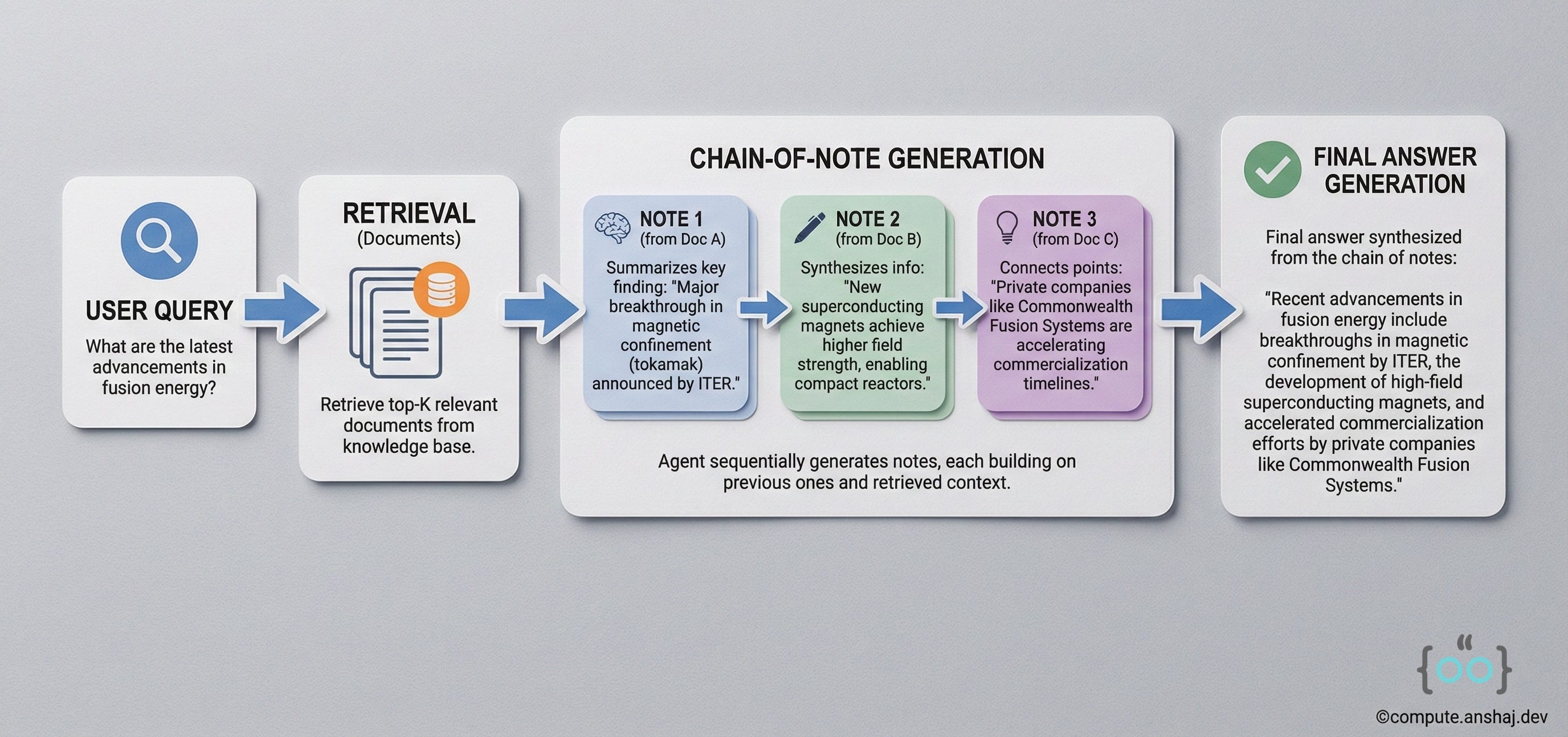
The CoN Solution: CoN forces the model to take notes before answering.
Read Doc 1: “This document talks about burgers. It is irrelevant to Mars.”
Read Doc 2: “This document discusses Mars geology. It mentions no monarchy.”
Synthesize: “Based on the notes, there is no information about a King of Mars. The retrieval results were irrelevant.”
This architecture drastically improves Robustness. It creates a “Null” state. It turns the model from a Sycohphant (always trying to please) into a Critic (assessing the validity of its own inputs).
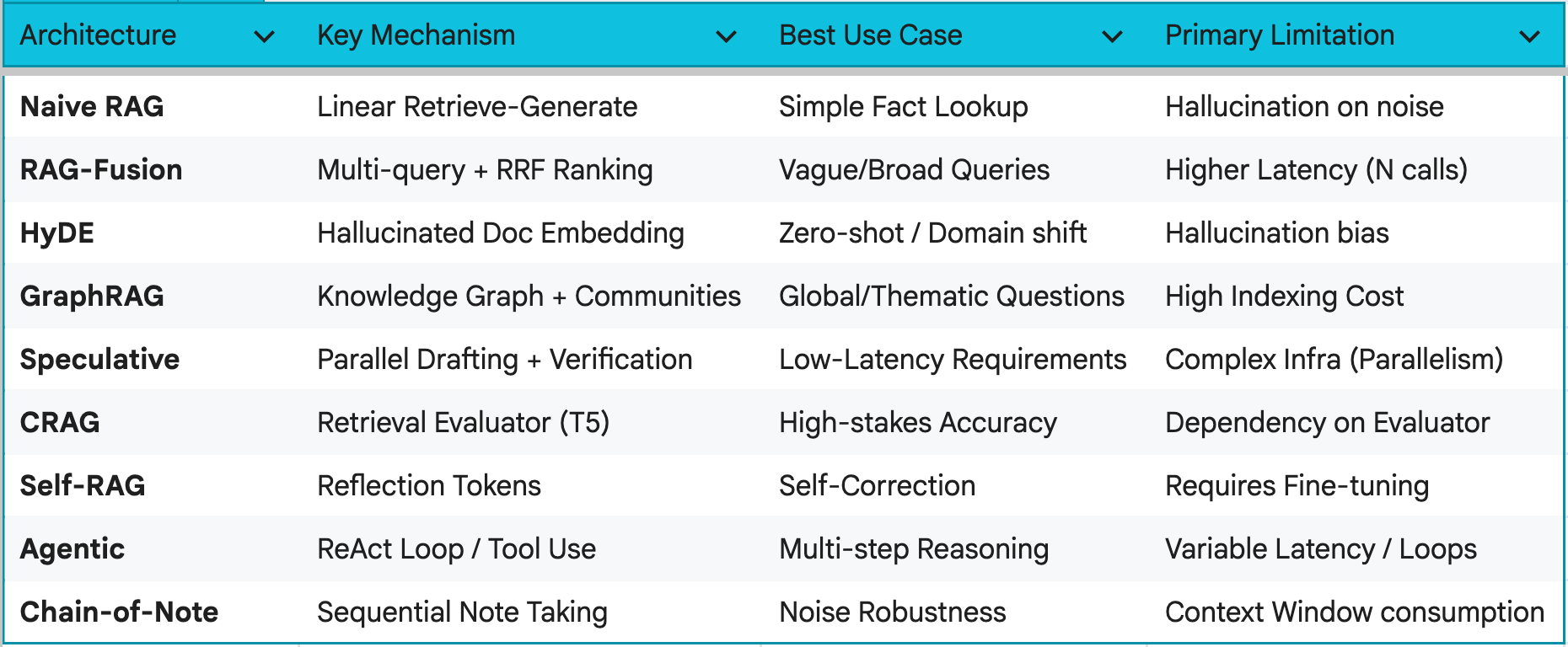
Choosing Your Stack
With so many architectures, how do you choose? Here is a comparison guide that can help.
The Gold Standard Stack
If you are building an enterprise RAG system today, a robust starting point is often a hybrid
Routing: Adaptive front-end (don’t RAG everything).
Retrieval: Hybrid Search (Vector + Keyword) with Reranking
Architecture: Modular. Start with a linear pipeline. Upgrade to Agentic only for specific complex query types (using the Router).
Database: A store that supports both Vector and Metadata filtering (e.g., Pinecone, Weaviate, or pgvector).
The Road Ahead
The days of pip install langchain; qa_chain.run() are over. RAG has matured into a serious systems engineering discipline.
We are moving towards Cognitive RAG: systems that model the user’s intent, structure the knowledge globally (Graphs), and reason iteratively (Agents). The trade-offs are no longer just about accuracy; they are about
Autonomy vs. Control
Latency vs. Depth.
As a developer, your job is no longer just to connect the LLM to the DB. It is to architect the flow of thought. Whether you choose the structural rigor of GraphRAG or the dynamic flexibility of Agentic RAG, the goal remains the same: building systems that don’t just retrieve data, but actually understand it.
Welcome to the next generation of Intelligent Information Retrieval. Thank you so much for reading this super-long post, and I hope you have a wonderful day.